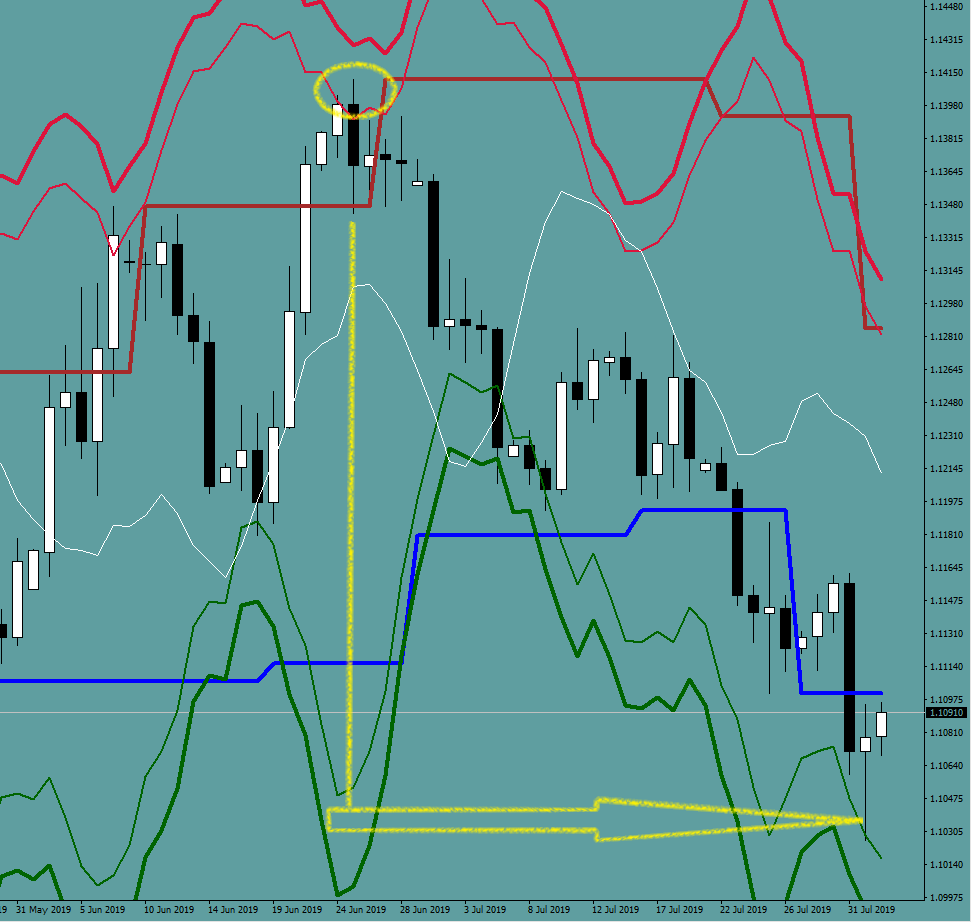
The concept of the energy bands is to attribute predicting power to the current consolidation level by showing how far the price could get if it was to keep on moving in a direction – before hitting an “exhaustion”.

Since somebody had to think of this, I did.

An exhaustion would prompt a consolidation: price would have to start moving sideways, backwards or something in between.

For the last time I would mention that price cannot simply always do what it wants.

Imagine the value of these bands when you are playing options strategies, such as an iron condor. You must know where to put on your spread if you don’t want it to become a liability.

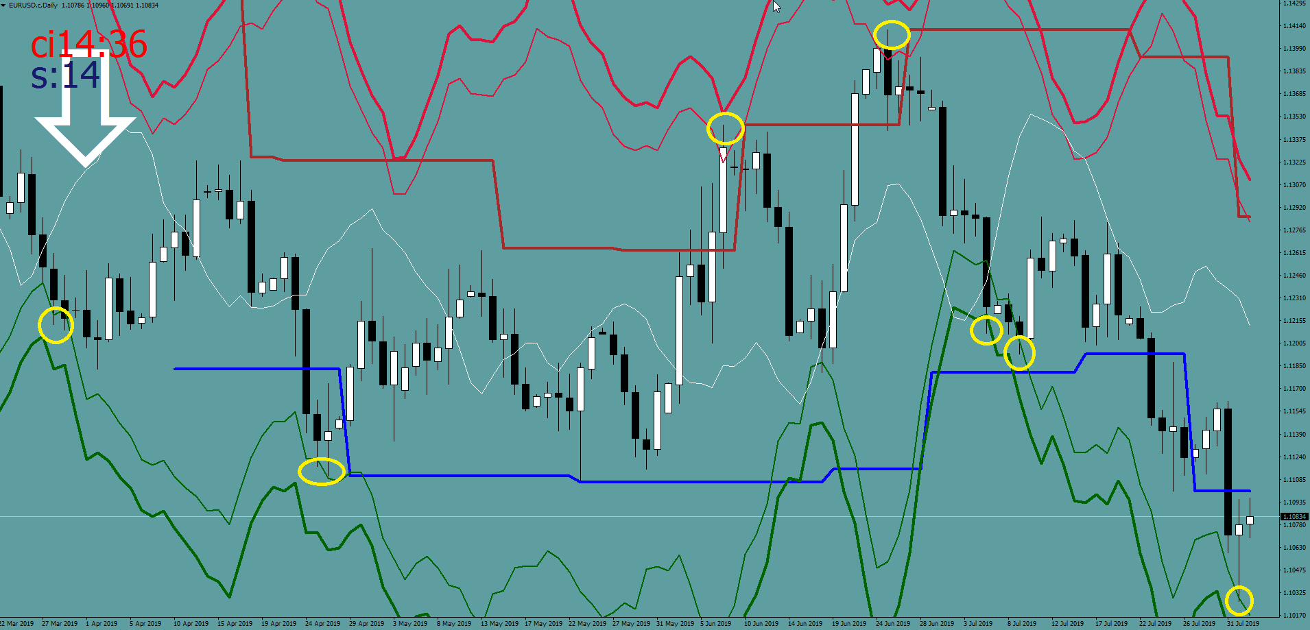
 cval[i] = (.0200/55)*adj*(ChoppinessIndex(ChoppinessPeriod,i+3)+ChoppinessIndex(ChoppinessPeriod,i+4)+ChoppinessIndex(ChoppinessPeriod,i+5))/3;

The consolidation value is derived from the mean of the 3rd, 4th and 5th, 14-sample consolidation values. The adjustment is 70%.

This value is added or subtracted from the average of the 8th, 7th and 5th high/low with an individual multiplier.

 c2[i] = (iLow(NULL,0,i+8)+iLow(NULL,0,i+7)+iLow(NULL,0,i+5))/3-cval[i]*1.28
+(VOLA-50)/10000;

double VOLA = (sqrt(252) * (log(iClose(NULL,0,0) / iClose(NULL,0,1)/5*1000)))+10;

The bands are asymmetric. How did I end up with 1.27 and 1.62 multiplier on the downside and 0.9 and 1.15 on the upside and with a 4th value thrown in for good measure, is a mystery.

What matters is that these bands are dynamic, and can land you the right idea of distance possibilities.

For instance, when the high was made, did you or did you not have the maximum likely travel distance at your hand, at that very moment?